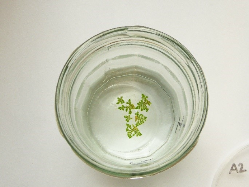
This dataset shows the effects of herbicides (detected in the Great Barrier Reef catchments) on growth rates (from surface area and biomass) and photosynthesis (effective quantum yield) on the aquatic fern Azolla pinnata during laboratory experiments conducted in 2019. The aims of this project were to develop and apply standard ecotoxicology protocols to determine the effects of Photosystem II (PSII) and alternative herbicides on the growth and photosynthetic efficiency of the aquatic fern Azolla pinnata. Growth bioassays were performed over 14-day exposures using herbicides that have been detected in the Great Barrier Reef catchment area (O’Brien et al. 2016). Chronic effects of herbicides on the photophysiology of A. pinnata, measured by chlorophyll fluorescence as the effective quantum yield (Delta F/Fm’) were investigated using PAM fluorometry after 14-day herbicide exposure. These toxicity data will enable improved assessment of the risks posed by PSII and alternative herbicides to aquatic macrophytes for both regulatory purposes and for comparison with other taxa. Methods: The aquatic fern Azolla pinnata was sourced from Watergarden Paradise Nursery, NSW. Cultures were established in IRRI2 medium (Pereira & Carrapiço 2009). Cultures were maintained in 10 L tubs containing 3–5 L IRRI2 as batch cultures with weekly transfers to fresh medium. Clean culture solutions were maintained at 26 ± 1 °C, under a 12:12 hr light:dark cycle (65-77µmol photons m–2 s–1). Herbicide stock solutions were prepared using PESTANAL (Sigma-Aldrich) analytical grade products (HPLC greater than or equal to 98%): diuron (CAS 330-54-1), fluometuron (CAS 2164-17-2), fluroxypyr (CAS 69377-81-7), haloxyfop-p-methyl (CAS 72619-32-0), imazapic (CAS 104098-48-8), isoxaflutole (CAS 141112-29-0) and triclopyr (CAS 5535-06-3). The selection of herbicides was based on application rates and detection in coastal waters of the GBR (Grant et al. 2017, O’Brien et al. 2016). Stock solutions were prepared in 100 mL glass volumetric flasks using milli-Q water. Diuron, haloxyfop-p-methyl and isoxaflutole were dissolved using analytical grade acetone (< 0.01% (v/v) in exposures). Imazapic was dissolved in methanol (less than 0.01% (v/v) in exposure). No solvent carrier was used for the preparation of the remaining herbicide stock solutions. Cultures of A. pinnata were exposed to a range of herbicide concentrations over a period of 14 days. Fronds were selected from actively growing cultures free of overt disease or deformity. Four triplicate fronds each comprising eight ramets were added to 100 mL of each herbicide solution concentration and control treatment. In each toxicity test, control (no herbicide) and solvent control (if used) treatments were added to support the validity of the test protocols and to monitor continued performance of the assays. Experiments were conducted in IRRI2 medium (Pereira & Carrapiço 2009) with solutions replaced at Day 7. Three replicates of each treatment solution and control were prepared and incubated at 26.6 ± 0.5 °C under a 12:12 h light:dark cycle (90 ± 6 µmol photons m–2 s–1). Each replicate treatment was photographed at a standard height to estimate surface area at Day 0 and Day 14. Biomass of a representative numbers of fronds were weighed to 4 significant figures using an analytical balance after blotting for 15 seconds to remove excess moisture. Fronds from each treatment replicate were weighed at Day 14 using the same technique. Specific growth rates (SGR) were expressed as the logarithmic increase in surface area or biomass from day i (ti) to day j (tj) as per equation (1), where SGRi-j is the specific growth rate from time i to j; Xj is the surface area or biomass at day j and Xi is the surface area or biomass at day i (OECD 2006). SGR i-j = [(ln Xj - ln Xi )/(tj - ti )] (day-1) SGR relative to the control / solvent control treatment was used to derive chronic effect values for growth inhibition. A test was considered valid, if the SGR for frond number or surface area of control replicates was greater than or equal to 0.0.0495 day-1 (OECD 2014). Physical and chemical characteristics of each treatment were measured at 0, 7 and 14 days on new and old treatment solutions for pH, electrical conductivity and temperature. Temperature was also logged in 15-min intervals over the total test duration. Analytical samples were taken at 0 and 14 days. Chronic effects of herbicides on the photophysiology of A. pinnata, measured by chlorophyll fluorescence as the effective quantum yield (Delta F/Fm’), were investigated at 14 days using PAM fluorometry (mini-PAM, Walz, Germany). Light adapted minimum fluorescence (F) and maximum fluorescence (Fm') were determined and effective quantum yield was calculated for each treatment as per equation (2)(Schreiber et al. 2002). Delta F/Fm’ = (Fm’-F)/Fm’ Mini- PAM settings were set to ETR-F = 0.84, F-Offset = 46, measuring light frequency = 3, measuring intensity = 4, gain = 2; damp = 3. Saturation pulse settings: intensity = 6, width = 0.6. Mean percent inhibition in SGR and Delta F/Fm’ of each treatment relative to the control treatment was calculated as per equation (3)(OECD 2006), where Xcontrol is the average SGR or Delta F/Fm’ of control and Xtreatment is the average SGR or Delta F/Fm’ of single treatments. % Inhibition = [(X control - X treatment )/X control] x 100 Format: Azolla pinnata herbicide toxicity data_eAtlas.xlsx Data Dictionary: There are two or three tabs for each herbicide in the spreadsheet. The first tab corresponds to the specific growth rate – surface area (SGR-SA) data; the second tab is biomass (SGR-B) data; and the pulse amplitude modulation (PAM) fluorometry data. The last tab of the dataset shows the measured water quality (WQ) parameters (pH, electrical conductivity and temperature) of each herbicide test. Where value equals '-', measurement not taken. Diu – Diuron Fluo - Fluometuron Flur - Fluroxypyr Halo – Haloxyfop Imaz - Imazapic Isox - Isoxaflutole Tri – Triclopyr For each ‘herbicide’_SGR tab: SGR = specific growth rate - the logarithmic increase from day 0 to day 14 as either surface area (SA) (mm2) or biomass (B) (g) Nominal (µg/L) = nominal herbicide concentrations used in the bioassays; SC denotes solvent control which is no herbicide and contains less than 0.01% v/v solvent carrier as per the treatments Measured (µg/L) = measured concentrations analysed by The University of Queensland Rep = replicate notation is 1-3 T14_Growth = surface area (mm2) or biomass (g) at day 14 ln(day14) = natural logarithm of surface area (mm2) or biomass (g) at day 14 Average T0_Growth = surface area (mm2) or biomass (g) at day 0 ln(day0) = natural logarithm of surface area (mm2) or biomass (g) at day 0 For each ‘herbicide’_PAM tab: PAM = pulse amplitude modulation fluorometry to calculate effective quantum yield (light adapted) Nominal (µg/L) = nominal herbicide concentrations used in the bioassays; SC denotes solvent control which is no herbicide and contains less than 0.01% v/v solvent carrier as per the treatments; Measured (µg/L) = measured concentrations analysed by The University of Queensland notation is 1-3; for PAM data, notation is 1-3 Delta F/Fm' = effective quantum (light adapted) yield measured by a Pulse Amplitude Modulation (PAM) fluorometer References: Grant, S., Gallen, C., Thompson, K., Paxman, C., Tracey, D. and Mueller, J. (2017) Marine Monitoring Program: Annual Report for inshore pesticide monitoring 2015-2016. Report for the Great Barrier Reef Marine Park Authority, Great Barrier Reef Marine Park Authority, Townsville, Australia. 128 pp, http://dspace-prod.gbrmpa.gov.au/jspui/handle/11017/13325 O’Brien, D., Lewis, S., Davis, A., Gallen, C., Smith, R., Turner, R., Warne, M., Turner, S., Caswell, S. and Mueller, J.F. (2016) Spatial and temporal variability in pesticide exposure downstream of a heavily irrigated cropping area: application of different monitoring techniques. Journal of Agricultural and Food Chemistry 64(20), 3975-3989. OECD (2006) Current approaches in the statistical analysis of ecotoxicity data. OECD Publishing. OECD (2014) Test No. 238: Sediment-Free Myriophyllum Spicatum Toxicity Test, OECD Guidelines for the Testing of Chemicals, Section 2, OECD Publishing, Paris. Pereira, A.L., and Carrapiço, F. (2009) Culture of Azolla filiculoides in artificial conditions. Plant Biosystems, 143(3), 431-434 Rueden, C.T., Schindelin, J., Hiner, M.C. et al. (2017) ImageJ2: ImageJ for the next generation of scientific image data. BMC Bioinformatics 18:529, PMID 29187165, doi:10.1186/s12859-017-1934-z Data Location: This dataset is filed in the eAtlas enduring data repository at: data\nesp3\3.1.5_Pesticide-guidelines-GBR

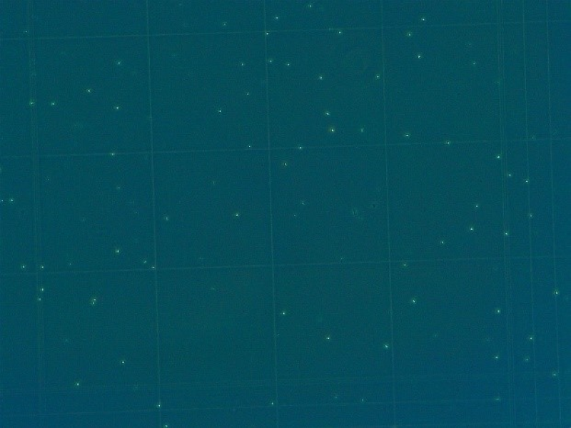
This dataset shows the effects of herbicides (detected in the Great Barrier Reef catchments) on the growth rates (from cell density data) and photosynthesis (effective quantum yield) on the microalgae Chlorella sp. during laboratory experiments conducted from 2017-2019. The aims of this project were to develop and apply standard ecotoxicology protocols to determine the effects of Photosystem II (PSII) and alternative herbicides on the growth and photosynthetic efficiency of the microalgae Chlorella sp. Growth bioassays were performed over 3-day exposures using herbicides that have been detected in the Great Barrier Reef catchment area (O’Brien et al. 2016). Effects of herbicides on the photophysiology of Chlorella sp., measured by chlorophyll fluorescence as the effective quantum yield (Delta F/Fm’) were investigated using mini-PAM fluorometry after 72 h herbicide exposure. These toxicity data will enable improved assessment of the risks posed by PSII and alternative herbicides to microalgae for both regulatory purposes and for comparison with other taxa. Methods: The chlorophyte Chlorella sp. was sourced from the Supervising Scientist, Department Energy and Environment, Darwin. Cultures of Chlorella sp. were established in MBL medium (Riethmuller et al 2003, Pease et al 2016). Cultures were maintained in sterile 250 mL Erlenmeyer flasks as batch cultures in exponential growth phase with weekly transfers of 1 - 3 mL of a 7 day-old Chlorella sp. suspension to 100 mL MBL medium under sterile conditions. Clean culture solutions were maintained at 26 ± 2°C, and under a 12:12 h light:dark cycle (91 ± 12 µmol photons m–2 s–1). Herbicide stock solutions were prepared using PESTANAL (Sigma-Aldrich) analytical grade products (HPLC greater than or equal to 98%): bromacil (CAS 314-40-9), diuron (CAS 330-54-1), haloxyfop-p-methyl (CAS 72619-32-0), hexazinone (CAS 51235-04-2), imazapic (CAS 104098-48-8), isoxaflutole (CAS 141112-29-0), prometryn (CAS 7287-19-6) and propazine (CAS 139-40-2). The selection of herbicides was based on application rates and detection in coastal waters of the GBR (Grant et al. 2017, O’Brien et al. 2016). Stock solutions were prepared in sterile 1 L glass Schott bottles using milli-Q water. Diuron, haloxyfop-p-methyl, hexazinone, isoxaflutole and prometryn were dissolved using analytical grade acetone (< 0.01% (v/v) in exposures). Imazapic was dissolved in methanol (less than or equal to 0.01% (v/v) in exposure). No solvent carrier was used for the preparation of the remaining herbicide stock solutions. Cultures of Chlorella sp. were exposed to a range of herbicide concentrations over a period of 72 h. Inoculum was taken from cultures in exponential growth phase (4 – 7 day-old cultures). A Chlorella sp. working suspension was prepared in a 100 mL volumetric flask. A 1:10 and 1:100 dilution was prepared and counted using a haemocytometer under a compound microscope to determine appropriate dilution volumes. The pre-determined inoculum was added to 50 mL of each test and control treatment replicates to the required dilution (3 – 3.1 x 104 cells/ mL). In each toxicity test, a control (no herbicide) and solvent control (if used) treatments were added to support the validity of the test protocols and to monitor continued performance of the assays. All treatment solutions were prepared in 0.5x strength MBL medium. Replicates were incubated at 26.6 ± 0.5 °C under a 12:12 h light:dark cycle (190 ± 14 µmol photons m–2 s–1). Sub-samples were taken from each replicate to measure cell densities of algal populations at 72 h using a haemocytometer and photographed under phase contrast conditions. Cell counts were done either manually or using imageJ from microscope photographs (Rueden et al 2017). Specific growth rates (SGR) were expressed as the logarithmic increase in cell density from day i (ti) to day j (tj) as per equation (1), where SGRi-j is the specific growth rate from time i to j; Xj is the cell density at day j and Xi is the cell density at day i (OECD 2011). SGR i-j = [(ln Xj - ln Xi )/(tj - ti )] (day-1) (1) SGR relative to the control treatment was used to derive chronic effect values for growth inhibition. A test was considered valid, if the SGR of control replicates was greater than or equal to 0.92 day-1 (OECD 2011). Physical and chemical characteristics of each treatment were measured at 0 h and 72 h including pH, electrical conductivity and temperature. Chamber temperature was also logged in 15-min intervals over the total test duration. Analytical samples were taken at 0 h and 72 h. Effects of herbicides on the photophysiology of Chlorella sp., measured by chlorophyll fluorescence as the effective quantum yield (Delta F/Fm’ ), were investigated at 72 h using mini-PAM fluorometry (mini-PAM, Walz, Germany). Light adapted minimum fluorescence (F) and maximum fluorescence (Fm’) were determined and effective quantum yield was calculated for each treatment as per equation (2)(Schreiber et al. 2002). Delta F/Fm’ = (Fm’-F)/Fm’ (2) Mini- PAM settings were set to ETR-F = 0.84, F-Offset = 92, measuring light frequency = 3, measuring intensity = 4, gain = 3; damp = 3. Saturation pulse settings: intensity = 6, width = 0.6. Mean percent inhibition in SGR and Delta F/Fm’ of each treatment relative to the control treatment was calculated as per equation (3)(OECD 2011), where Xcontrol is the average SGR or Delta F/Fm’ of control and Xtreatment is the average SGR or Delta F/Fm’ of single treatments. % Inhibition = [(X control - X treatment )/X control] x 100 (3) Format: Chlorella sp.herbicide toxicity data_eAtlas.xlsx Data Dictionary: There are two tabs for each herbicide in the spreadsheet. The first tab corresponds to the specific growth rate (SGR) data; the second tab is the pulse amplitude modulation (PAM) fluorometry data. The last tab of the dataset shows the measured water quality (WQ) parameters (pH, electrical conductivity and temperature) of each herbicide test. Brom - Bromacil Diu – Diuron Halo – Haloxyfop Hex - Hexazinone Imaz – Imazapic Isox - Isoxaflutole Prom - Prometryn Prop - Propazine For each ‘herbicide’_SGR tab: SGR = specific growth rate – the logarithmic increase from day 0 to day 3 Nominal (µg/L) = nominal herbicide concentrations used in the bioassays; SC denotes solvent control which is no herbicide and contains less than 0.01% v/v solvent carrier as per the treatments Measured (µg/L) = measured concentrations analysed by The University of Queensland Rep = Replicate: for SGR, notation is 1-3; for PAM data, notation is 1-3 T3_CellsPerMl = cell density at day 3 ln(day3) = natural logarithm of cell density at day 3 Average T0_CellsPerMl = average cell density at day 0 ln(Day0) = natural logarithm of cell density at day 0 For each ‘herbicide’_PAM tab: PAM = pulse amplitude modulated fluorometry to calculate effective quantum yield (light adapted) Nominal (µg/L) = nominal herbicide concentrations used in the bioassays; SC denotes solvent control which is no herbicide and contains less than 0.01% v/v solvent carrier as per the treatments Measured (µg/L) = measured concentrations analysed by The University of Queensland Rep = Replicate: for SGR, notation is 1-3; for PAM data, notation is 1-3 Delta F/Fm’ = effective quantum (light adapted) yield measured by a Pulse Amplitude Modulation (PAM) fluorometer References: Grant, S., Gallen, C., Thompson, K., Paxman, C., Tracey, D. and Mueller, J. (2017) Marine Monitoring Program: Annual Report for inshore pesticide monitoring 2015-2016. Report for the Great Barrier Reef Marine Park Authority, Great Barrier Reef Marine Park Authority, Townsville, Australia. 128 pp, http://dspace-prod.gbrmpa.gov.au/jspui/handle/11017/13325 O’Brien, D., Lewis, S., Davis, A., Gallen, C., Smith, R., Turner, R., Warne, M., Turner, S., Caswell, S. and Mueller, J.F. (2016) Spatial and temporal variability in pesticide exposure downstream of a heavily irrigated cropping area: application of different monitoring techniques. Journal of Agricultural and Food Chemistry 64(20), 3975-3989. OECD (2011) OECD guidelines for the testing of chemicals: freshwater alga and cyanobacteria, growth inhibition test, Test No. 201. https://search.oecd.org/env/test-no-201-alga-growth-inhibition-test-9789264069923-en.htm (accessed 28 August 2019). Pease C, Mooney T, Trenfield M, Costello C & Harford A (2016). Updated procedure for the 72 hour algal growth inhibition toxicity test using Chlorella sp. Internal Report 645, September, Supervising Scientist, Darwin Riethmuller, N., Camilleri, C., Franklin, N., Hogan, A., King, A., Koch, A., Markich, S.J., Turley, C. and van Dam, R. (2003) Ecotoxicological testing protocols for Australian tropical freshwater ecosystems. Supervising Scientist Report 173, Supervising Scientist, Darwin NT. Rueden, C.T., Schindelin, J., Hiner, M.C. et al. (2017) ImageJ2: ImageJ for the next generation of scientific image data. BMC Bioinformatics 18:529, PMID 29187165, doi:10.1186/s12859-017-1934-z Data Location: This dataset is filed in the eAtlas enduring data repository at: data\nesp3\3.1.5_Pesticide-guidelines-GBR

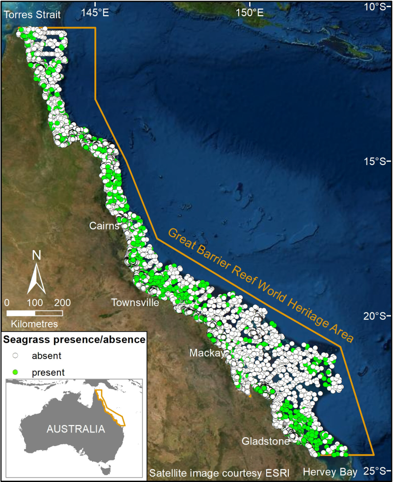
This dataset summarises 35 years of seagrass data collection (1984-2018) within the Great Barrier Reef World Heritage Area into one GIS shapefile containing seagrass presence and absence survey data for 81,387 sites. Managing seagrass resources in the GBRWHA requires adequate baseline information on where seagrass is (presence/absence), what species are present, and date of collection. This baseline is particularly important as a reference point against which to compare seagrass loss or change through time. The scale of the GBRWHA (1000s of kilometres) and the remoteness of many seagrass meadows from human populations present a challenge for research and management agencies reporting on the state of seagrass ecological indicators. Broad-scale and repeated surveys/studies of areas this large are logistically and financially impracticable. However seagrass data is being collected through various projects which, although designed for specific reasons, are amenable to collating a picture of the extent and state of the seagrass resource. James Cook University’s Centre for Tropical Water & Aquatic Ecosystem Research (TropWATER) Seagrass Group (The Seagrass Group was part of the Queensland Government Department of Fisheries prior to 2013) has been collecting spatial data on GBR seagrass since the early 1980s. In this project TropWATER updated a previous synthesis of seagrass site data (NESP Project 3.1: https://eatlas.org.au/data/uuid/77998615-bbab-4270-bcb1-96c46f56f85a), with more recent data collected 2014-2018 to make this publicly available. Data included here from Cleveland Bay was used to classify seagrass community types, set desired state targets and for connecting sediment load targets to ecological outcomes for seagrass (NESP Project 3.2.1). In making this data publicly available for management, the authors from the TropWATER Seagrass Group request being contacted and involved in decision making processes that incorporate this data, to ensure its limitations are fully understood. Methods: The sampling methods used to study, describe and monitors seagrass meadows were developed by the TropWATER Seagrass Group and tailored to the location and habitat surveyed; these are described in detail in the relevant publications (https://research.jcu.edu.au/tropwater). Methods for data sets collected by CSIRO are reported in Pitcher et al (2007). 1. Location – Latitudes and longitudes are from converted RADAR fix or GPS. 2. Depth – Depth for subtidal sites only estimated for each site using Beaman, R.J. (2017): High-resolution depth model for the Great Barrier Reef - 30 m (http://pid.geoscience.gov.au/dataset/115066). Depth for intertidal sites = 0. 3. Sediment – Dominant sediment type from deck description. 4. Seagrass metrics –Observers recorded seagrass presence/absence and presence/absence of each seagrass species using video transects, grabs, free diving, helicopter and walking: - Video transect: Commonly used for subtidal meadows at each transect site. A CCTV camera was lowered to the bottom and towed at drift speed (less than one knot) for approximately 100m. Latitude/longitude represent the start of each transect. Footage was observed on a TV monitor and digitally recorded. The recording was paused at random times and frames selected to determine presence/absence for seagrass and each seagrass species. The camera sled included a small collecting net to obtain a specimen for identification. - van Veen grab: Commonly used for subtidal meadows. A sample of seagrass was collected using a van Veen grab (grab area 0.0625 m2) to determine presence/absence for seagrass and each seagrass species at each site. - Free diving, helicopter and walking: Presence/absence for seagrass and each seagrass species was estimated at each site, with a site representing approximately 10m2. Geographic Information System (GIS) All survey data were entered into a Geographic Information System (GIS) using MapInfo (generally pre-2005) then ArcMap® software. MapInfo spatial data was converted to ArcMap shapefiles. The GIS layer is a point (site) layer with a projected coordinate system of GDA94. Seagrass site layer This layer contains information on all data collected at assessment sites, and includes: 1. Temporal survey details – month and year when the survey occurred; 2. Spatial survey details – latitude/longitude, intertidal/subtidal, site depth in metres below mean sea level for subtidal sites; 3. Seagrass information including presence/absence of seagrass, and for each of 12 seagrass species; 4. Dominant sediment type; 5. Survey name; and 6. Sampling methods – helicopter, walking, boat with camera, diver, grab and/or sled. Spatial limits Seagrass data north and south of the GBRWHA were excluded from the layers and are held by TropWATER, JCU. Data were included when sites extended west of the GBRWHA boundary into coastal and estuarine water immediately adjacent. Modelled distributions are available (Coles et al 2009; Pitcher et al 2007) but not included here. Taxonomy Seagrass taxonomy has changed through time, with species such as Halophila ovata no longer recognised and some doubts expressed about other species whose morphology is relatively plastic. Field surveys have at times grouped species that are difficult to distinguish outside a laboratory. To address these issues we have amalgamated some species into complexes: Halophila ovata, Halophila minor, Halophila colesi/australis and Halophila ovalis are included as Halophila ovalis. Halodule pinifolia is grouped with Halodule uninervis. Data collected in winter may underestimate the extent of ephemeral species such as Halophila decipiens and Halophila tricostata. This is important if this composite is used to compare annual changes. Zostera muelleri subsp. capricorni has been abbreviated to Zostera capricorni throughout. Base map The base map used is courtesy ESRI 2020. Since the original surveys in 1980 there have been numerous changes to the shoreline, the most obvious being seaward encroachment of mangrove forests and reclamation for marina and coastal development. We have not edited seagrass sites to prevent older data from overlapping these features. Data sets Spatial data from over 200 site layers are included in this composite. Further information can be found in this publication: Carter, A. B., McKenna, S. A., Rasheed, M. A., McKenzie L, Coles R. G. (2016) Seagrass mapping synthesis: A resource for coastal management in the Great Barrier Reef World Heritage Area. Report to the National Environmental Science Programme. Reef and Rainforest Research Centre Limited, Cairns (22 pp). Available at http://nesptropical.edu.au/wp-content/uploads/2016/03/NESP-TWQ-3.1-FINAL-REPORT.pdf and Lambert, V., Collier, C., Brodie, J., Adams, M.P., Baird, M., Bainbridge, Z., Carter, A., Lewis, S., Rasheed, M., Saunders, M., O’Brien, K., (2020) Connecting Sediment Load Targets to Ecological Outcomes for Seagrass. Report to the National Environmental Science Program. Reef and Rainforest Research Centre Limited, Cairns (140pp.). Limitations of the Data: Data included extends back to the mid-1980s. Large parts of the coast have not been mapped for seagrass presence since that time. Technology and methods for mapping and position fixing have improved dramatically in 30 years. This layer represents the most reliable interpretation of that early data. Spatial Extent: Seagrass data north and south of the GBRWHA were excluded from the layers. No seagrass site data exists east of the GBRWHA boundary. Data were included when sites extended west of the GBRWHA boundary into coastal and estuarine water immediately adjacent. Modelled distributions are available (Coles et al 2009; Pitcher et al 2007) but not included here. Format: This dataset consists of a point shapefile with a geographic coordinate system of GDA94. The site layer has been saved as a layer package with symbology representing seagrass presence/absence (Seagrass_sites_1984_2018.lpk) Seagrass site Data: - MONTH: Month of survey. - YEAR: Year of survey. - SURVEY_NAM: Description of the location of the survey. - LATITUDE/LONGITUDE: survey site. Seagrass information: - PRESENCE_A: the presence/absence of seagrass where Yes = presence and No = absence. - C_ROTUNDAT: presence/absence of Cymodocea Rotundata at the site. - C_SERRULAT: presence/absence of Cymodocea Serrulata at the site. - E_ACOROIDE: presence/absence of Enhalus Acoroides at the site. - H_CAPRICOR: presence/absence of Halophila Capricorni at the site. - H_DECIPIEN: presence/absence of Halophila Decipiens at the site. - H_OVALIS: presence/absence of Halophila Ovalis at the site. - H_SPINULOS: presence/absence of Halophila Spinulosa at the site. - H_TRICOSTA: presence/absence of Halophila Tricostata at the site. - H_UNINERVI: presence/absence of Halodule Uninervis at the site. - S_ISOETIFO: presence/absence of Syringodium Isoetifolium at the site. - T_CILIATUM: presence/absence of Thalassodendron Ciliatum at the site. - T_HEMPRICH: presence/absence of Thalassia Hemprichii at the site. - Z_CAPRICOR: presence/absence of Zostera Muelleri subsp. Capricorni at the site. Additional site information: - SEDIMENT: predominant type of sediment at the location, mud, gravel, reef, rock, rubble, sand, shell or not recorded. - SURVEY_MET: helicopter, walking, boat with camera, diver, grab and/or sled - TIDAL: intertidal or subtidal seabed at site - DEPTH: the site depth in metres below mean sea level (dbMSL). References: Carter, A. B., McKenna, S. A., Rasheed, M. A., McKenzie L, Coles R. G. (2016) Seagrass mapping synthesis: A resource for coastal management in the Great Barrier Reef World Heritage Area. Report to the National Environmental Science Programme. Reef and Rainforest Research Centre Limited, Cairns (22 pp). Available at http://nesptropical.edu.au/wp-content/uploads/2016/03/NESP-TWQ-3.1-FINAL-REPORT.pdf Lambert, V., Collier, C., Brodie, J., Adams, M.P., Baird, M., Bainbridge, Z., Carter, A., Lewis, S., Rasheed, M., Saunders, M., O’Brien, K., (2020) Connecting Sediment Load Targets to Ecological Outcomes for Seagrass. Report to the National Environmental Science Program. Reef and Rainforest Research Centre Limited, Cairns (140pp.). Data Location: This dataset is filed in the eAtlas enduring data repository at: data\NESP3\3.2.1_Eco-load-targets-seagrass

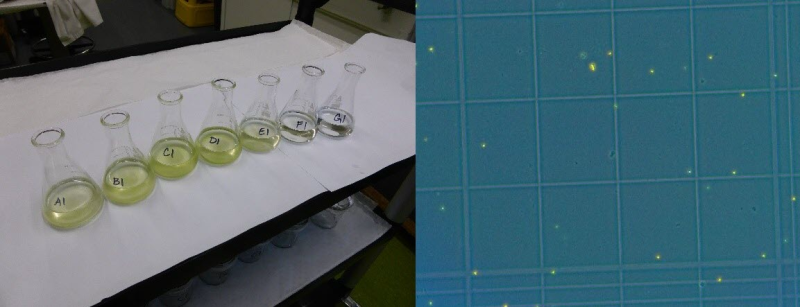
This dataset shows the effects of herbicides (detected in the Great Barrier Reef catchments) on the growth rates (from cell density data) and photosynthesis (effective quantum yield) on the green algae Desmodesmus asymmetricus during laboratory experiments conducted during 2019. The aims of this project were to develop and apply standard ecotoxicology protocols to determine the effects of Photosystem II (PSII) and alternative herbicides on the growth and photosynthetic efficiency of the green algae Desmodesmus asymmetricus. Growth bioassays were performed over 3-day exposures using herbicides that have been detected in the Great Barrier Reef catchment area (O’Brien et al. 2016). Effects of herbicides on the photophysiology of Desmodesmus asymmetricus, measured by chlorophyll fluorescence as the effective quantum yield (Delta F/Fm') were investigated using mini-PAM fluorometry after 72 h herbicide exposure. These toxicity data will enable improved assessment of the risks posed by PSII and alternative herbicides to microalgae for both regulatory purposes and for comparison with other taxa. Methods: The chlorophyte Desmodesmus asymmetricus was purchased from the Australian National Algae Supply Service, Hobart (CSIRO). Cultures of Desmodesmus asymmetricus were established in MLA medium (Bolch and Blackburn 1996). Cultures were maintained in sterile 250 mL Erlenmeyer flasks as batch cultures in exponential growth phase with weekly transfers of 1 - 3 mL of a 7 day-old Desmodesmus asymmetricus suspension to 100 mL MLA medium under sterile conditions. Clean culture solutions were maintained at 26 ± 2°C, and under a 12:12 h light:dark cycle (91 ± 12 µmol photons m–2 s–1). Herbicide stock solutions were prepared using PESTANAL (Sigma-Aldrich) analytical grade products (HPLC greater than or equal to 98%): bromacil (CAS 314-40-9), diuron (CAS 330-54-1), haloxyfop-p-methyl (CAS 72619-32-0), hexazinone (CAS 51235-04-2), imazapic (CAS 104098-48-8), isoxaflutole (CAS 141112-29-0), and propazine (CAS 139-40-2). The selection of herbicides was based on application rates and detection in coastal waters of the GBR (Grant et al. 2017, O’Brien et al. 2016). Stock solutions were prepared in sterile 100 - 500 mL glass volumetric flasks using milli-Q water. Diuron, haloxyfop-p-methyl, hexazinone and isoxaflutole were dissolved using analytical grade acetone (< 0.01% (v/v) in exposures). Imazapic was dissolved in methanol (less than or equal to 0.01% (v/v) in exposure). No solvent carrier was used for the preparation of the remaining herbicide stock solutions. Cultures of Desmodesmus asymmetricus were exposed to a range of herbicide concentrations over a period of 72 h. Inoculum was taken from cultures in exponential growth phase (4 – 7 day-old cultures). A Desmodesmus asymmetricus working suspension was prepared in a 100 ml volumetric flask. A 1:10 and 1:100 dilutions were prepared and counted using a haemocytometer under a compound microscope to determine appropriate dilution volumes. The pre-determined inoculum was added to 50 mL of each test and control treatment replicates to the required dilution (3 – 3.1 x 104 cells/ mL). In each toxicity test, a control (no herbicide) and solvent control (if used) treatments were added to support the validity of the test protocols and to monitor continued performance of the assays. All treatment concentrations were prepared in 0.5x strength MLA medium. Replicates were incubated at 26.6 ± 0.5 °C under a 12:12 h light:dark cycle (190 ± 14 µmol photons m–2 s–1). Sub-samples were taken from each replicate to measure cell densities of algal populations at 72 h using a haemocytometer and photographed under phase contrast conditions. Cell counts were done either manually or using imageJ from microscope photographs (Rueden et al 2017). Specific growth rates (SGR) were expressed as the logarithmic increase in cell density from day i (ti) to day j (tj) as per equation (1), where SGRi-j is the specific growth rate from time i to j; Xj is the cell density at day j and Xi is the cell density at day i (OECD 2011). SGR i-j = [(ln Xj - ln Xi )/(tj - ti )] (day-1) (1) SGR relative to the control treatment was used to derive chronic effect values for growth inhibition. A test was considered valid, if the SGR of control replicates was greater than or equal to 0.92 day-1 (OECD 2011). Physical and chemical characteristics of each treatment were measured at 0 h and 72 h including pH, electrical conductivity and temperature. Chamber temperature was also logged in 15-min intervals over the total test duration. Analytical samples were taken at 0 h and 72 h. Effects of herbicides on the photophysiology of Desmodesmus asymmetricus, measured by chlorophyll fluorescence as the effective quantum yield (Delta F/Fm'), were investigated at 72 h using mini-PAM fluorometry (mini-PAM, Walz, Germany). Light adapted minimum fluorescence (F) and maximum fluorescence (Fm') were determined and effective quantum yield was calculated for each treatment as per equation (2)(Schreiber et al. 2002). Delta F/Fm’ = (Fm’-F)/Fm’ (2) Mini- PAM settings were set to ETR-F = 0.84, F-Offset = 92, measuring light frequency = 3, measuring intensity = 4, gain = 3; damp = 3. Saturation pulse settings: intensity = 6, width = 0.6. Mean percent inhibition in SGR and Delta F/Fm' of each treatment relative to the control treatment was calculated as per equation (3)(OECD 2011), where Xcontrol is the average SGR or Delta F/Fm' of control and Xtreatment is the average SGR or Delta F/Fm' of single treatments. % Inhibition = [(Xcontrol - Xtreatment ) / Xcontrol] x 100 (3) Format: Desmodesmus asymmetricus herbicide toxicity data_eAtlas.xlsx Data Dictionary: There are two tabs for each herbicide in the spreadsheet. The first tab corresponds to the specific growth rate (SGR) data; the second tab is the pulse amplitude modulation (PAM) fluorometry data. The last tab of the dataset shows the measured water quality (WQ) parameters (pH, electrical conductivity and temperature) of each herbicide test. Where value equals '-', measurement not taken. Brom - Bromacil Diu – Diuron Halo – Haloxyfop Hex - Hexazinone Imaz – Imazapic Isox - Isoxaflutole Prop - Propazine For each ‘herbicide’_SGR tab: SGR = specific growth rate – the logarithmic increase from day 0 to day 3 Nominal (µg/L) = nominal herbicide concentrations used in the bioassays; SC denotes solvent control which is no herbicide and contains less than 0.01% v/v solvent carrier as per the treatments Measured (µg/L) = measured concentrations analysed by The University of Queensland Rep = Replicate: for SGR, notation is 1-3; for PAM data, notation is 1-3 T3_CellsPerMl = cell density at day 3 ln(day3) = natural logarithm of cell density at day 3 Average T0_CellsPerMl = average cell density at day 0 ln(Day0) = natural logarithm of cell density at day 0 For each ‘herbicide’_PAM tab: PAM = pulse amplitude modulated fluorometry to calculate effective quantum yield (light adapted) Nominal (µg/L) = nominal herbicide concentrations used in the bioassays; SC denotes solvent control which is no herbicide and contains less than 0.01% v/v solvent carrier as per the treatments Measured (µg/L) = measured concentrations analysed by The University of Queensland Rep = Replicate: for SGR, notation is 1-3; for PAM data, notation is 1-3 Delta F/Fm' = effective quantum (light adapted) yield measured by a Pulse Amplitude Modulation (PAM) fluorometer References: Bolch, C. J. S. and Blackburn S. I. (1996). Isolation and purification of Australian isolates of the toxic cyanobacterium Microcystis aeruginosa Kütz. Journal of Applied Phycology 8, 5-13 Grant, S., Gallen, C., Thompson, K., Paxman, C., Tracey, D. and Mueller, J. (2017) Marine Monitoring Program: Annual Report for inshore pesticide monitoring 2015-2016. Report for the Great Barrier Reef Marine Park Authority, Great Barrier Reef Marine Park Authority, Townsville, Australia. 128 pp, http://dspace-prod.gbrmpa.gov.au/jspui/handle/11017/13325 O’Brien, D., Lewis, S., Davis, A., Gallen, C., Smith, R., Turner, R., Warne, M., Turner, S., Caswell, S. and Mueller, J.F. (2016) Spatial and temporal variability in pesticide exposure downstream of a heavily irrigated cropping area: application of different monitoring techniques. Journal of Agricultural and Food Chemistry 64(20), 3975-3989. OECD (2011) OECD guidelines for the testing of chemicals: freshwater alga and cyanobacteria, growth inhibition test, Test No. 201. https://search.oecd.org/env/test-no-201-alga-growth-inhibition-test-9789264069923-en.htm (accessed 28 August 2019). Rueden, C.T., Schindelin, J., Hiner, M.C. et al. (2017) ImageJ2: ImageJ for the next generation of scientific image data. BMC Bioinformatics 18:529, PMID 29187165, doi:10.1186/s12859-017-1934-z Data Location: This dataset is filed in the eAtlas enduring data repository at: data\nesp3\3.1.5_Pesticide-guidelines-GBR

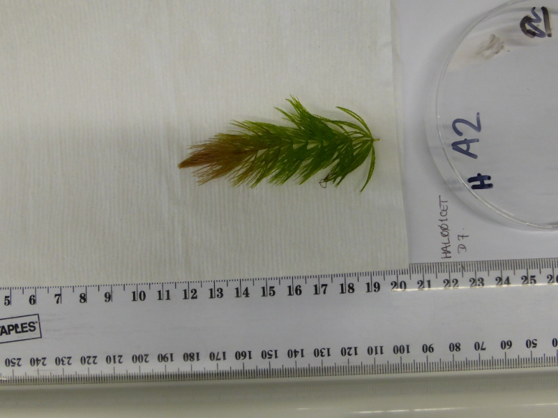
This dataset shows the effects of herbicides (detected in the Great Barrier Reef catchments) on the growth rates (from stem length and biomass) on the stonewort Ceratophyllum demersum during laboratory experiments conducted in 2019. The aims of this project were to develop and apply standard ecotoxicology protocols to determine the effects of non-PSII herbicides on the growth of the stonewort Ceratophyllum demersum. Growth bioassays were performed over 7-day exposures using herbicides that have been detected in the Great Barrier Reef catchment area (O’Brien et al. 2016). This toxicity data will enable improved assessment of the risks posed by non-PSII herbicides to aquatic macrophytes for both regulatory purposes and for comparison with other taxa. Methods: The stonewort Ceratophyllum demersum was supplied by Watergarden Paradise Aquatic Nursery, Bass Hill, NSW. Cultures were maintained in 500 L outdoor plastic tanks in recirculating dechlorinated tap water, aerated and maintained at ambient outdoor temperature and lighting. Test replicates selected 48 h in advance and acclimated in dechlorinated tap water, 26 ± 2 °C, under a 12:12 hr light:dark cycle (102 ± 9 µmol photons m–2 s–1). Herbicide stock solutions were prepared using PESTANAL (Sigma-Aldrich) analytical grade products (HPLC less than or equal to 98%): haloxyfop-p-methyl (CAS 72619-32-0), imazapic (CAS 104098-48-8) and triclopyr (CAS 5535-06-3). The selection of herbicides was based on application rates and detection in coastal waters of the GBR (Grant et al. 2017, O’Brien et al. 2016). Stock solutions were prepared in 500 mL glass volumetric flasks using milli-Q water. Haloxyfop-p-methyl was dissolved using analytical grade acetone (< 0.01% (v/v) in exposures). Imazapic was dissolved in methanol (less than or equal to 0.01% (v/v) in exposure). No solvent carrier was used for the preparation of triclopyr. Cultures of Ceratophyllum demersum were exposed to a range of herbicide concentrations over a period of 7 days. Plants were sourced from actively growing cultures free of overt disease or deformity. Individual plants approximately 35 mm long with 5 whorls and an apical tip were added to 150 mL of each herbicide solution concentration and control treatment. In each toxicity test, a control (no herbicide) and solvent control (if used) treatments were added to support the validity of the test protocols and to monitor continued performance of the assays. Experiments were conducted in autoclaved, recirculating dechlorinated tap water. Five replicates of each treatment solution and control were prepared and incubated at 26.6 ± 0.5 °C under a 12:12 h light:dark cycle (90 ± 6 µmol photons m–2 s–1). Each replicate treatment was photographed at a standard height to measure stem length at Day 0 and Day 7. Biomass of a representative numbers of fronds were weighed at Day 0 to 3 significant figures using an analytical balance after blotting for 15 seconds to remove excess moisture. Fronds from each treatment replicate were weighed at Day 7 using the same technique. Specific growth rates (SGR) were expressed as the logarithmic increase in stem length (mm) or biomass (g) from day i (ti) to day j (tj) as per equation (1), where SGRi-j is the specific growth rate from time i to j; Xj is the stem length or biomass at day j and Xi is the stem length or biomass at day i (OECD 2006). SGRi-j =[(ln Xj - ln X i) / (tj - ti)] (day-1) (1) SGR relative to the control / solvent control treatment was used to derive chronic effect values for growth inhibition. A test was considered valid, if the SGR for frond number or surface area of control replicates was greater than or equal to 0.0495 day-1 determined from (OECD 2006 and Riethmuller et al 2003). Physical and chemical characteristics of each treatment were measured at 0 and 7 days including pH, electrical conductivity and temperature. Temperature was also logged in 15-min intervals over the total test duration. Analytical samples were taken at 0 and 7 days. Format: Ceratophyllum demersum herbicide toxicity data_eAtlas.xlsx Data Dictionary: There are one or two tabs for each herbicide in the spreadsheet. The first tab corresponds to the specific growth rate – biomass (SGR-B) data; the second tab is stem length (SGR-L) data. The last tab of the dataset shows the measured water quality (WQ) parameters (pH, electrical conductivity and temperature) of each herbicide test. Halo – Haloxyfop Imaz – Imazapic Tri – Triclopyr For each ‘herbicide’_SGR tab: SGR = specific growth rate – the logarithmic increase from day 0 to day 7 as either biomass (B) (g/day) or stem length (L) (mm/day) Nominal (µg/L) = nominal herbicide concentrations used in the bioassays; SC denotes solvent control which is no herbicide and contains less than 0.01% v/v solvent carrier as per the treatments Measured (µg/L) = measured concentrations analysed by The University of Queensland Rep = Replicate: for SGR, notation is 1-5 T7_Biomass or Length = Biomass or Stem Length at Day 7 ln(day7) = natural logarithm of biomass (g) or stem length (mm) at Day 7 T0_Surface Area or Frond = Biomass (g) or Stem Length (mm) at Day 0 ln(day0) = natural logarithm of biomass (g) or stem length (mm) at Day 0 References: Grant, S., Gallen, C., Thompson, K., Paxman, C., Tracey, D. and Mueller, J. (2017) Marine Monitoring Program: Annual Report for inshore pesticide monitoring 2015-2016. Report for the Great Barrier Reef Marine Park Authority, Great Barrier Reef Marine Park Authority, Townsville, Australia. 128 pp, http://dspace-prod.gbrmpa.gov.au/jspui/handle/11017/13325 O’Brien, D., Lewis, S., Davis, A., Gallen, C., Smith, R., Turner, R., Warne, M., Turner, S., Caswell, S. and Mueller, J.F. (2016) Spatial and temporal variability in pesticide exposure downstream of a heavily irrigated cropping area: application of different monitoring techniques. Journal of Agricultural and Food Chemistry 64(20), 3975-3989. OECD (2006) Current approaches in the statistical analysis of ecotoxicity data. OECD Publishing. OECD (2014) Test Guideline 238: Sediment-free Myriophyllum spicatum toxicity test, OECD Publishing, Paris. Riethmuller, N., Camilleri, C., Franklin, N., Hogan, A., King, A., Koch, A., Markich, S.J., Turley, C. and van Dam, R. (2003) Ecotoxicological testing protocols for Australian tropical freshwater ecosystems. Supervising Scientist Report 173, Supervising Scientist, Darwin NT. Data Location: This dataset is filed in the eAtlas enduring data repository at: data\nesp3\3.1.5_Pesticide-guidelines-GBR

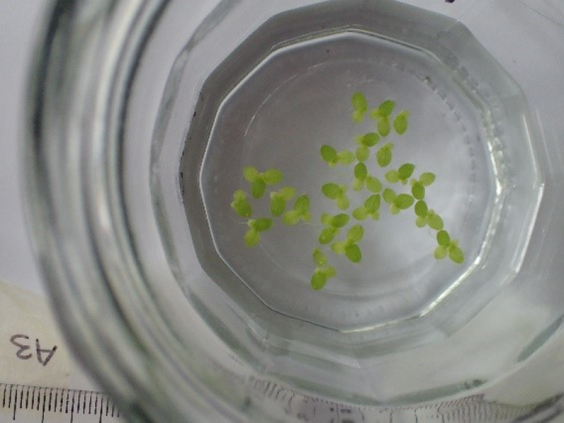
This dataset shows the effects of herbicides (detected in the Great Barrier Reef catchments) on the growth rates (from frond number and surface area) and photosynthesis (effective quantum yield) on the duckweed Lemna aequinoctialis during laboratory experiments conducted from 2017-2019. The aims of this project were to develop and apply standard ecotoxicology protocols to determine the effects of Photosystem II (PSII) and alternative herbicides on the growth and photosynthetic efficiency of the lesser duckweed Lemna aequinoctialis. Growth bioassays were performed over 4-day exposures using herbicides that have been detected in the Great Barrier Reef catchment area (O’Brien et al. 2016). Chronic effects of herbicides on the photophysiology of L. aequinoctialis, measured by chlorophyll fluorescence as the effective quantum yield (Delta F/Fm') were investigated using mini-PAM fluorometry after 4-day herbicide exposure. These toxicity data will enable improved assessment of the risks posed by PSII and alternative herbicides to aquatic macrophytes for both regulatory purposes and for comparison with other taxa. Methods: The lesser duckweed Lemna aequinoctialis was supplied by the Supervising Scientist, Department Agriculture, Water & Environment, Darwin, N.T.). Cultures were established in 0.5x strength CAAC medium (Riethmuller et al 2003; Pease et al 2016). Cultures were maintained in sterile 250 mL Erlenmeyer flasks as batch cultures with weekly transfers of 5-10 triplicate fronds to 100 mL 0.5x strength CAAC medium under sterile conditions. Clean culture solutions were maintained at 26 ± 2°C under a 12:12 h light:dark cycle (41 ± 5 µmol photons m–2 s–1). Herbicide stock solutions were prepared using PESTANAL (Sigma-Aldrich) analytical grade products (HPLC greater than or equal to 98%): bromacil (CAS 314-40-9); diuron (CAS 330-54-1), fluroxypyr (CAS 69377-81-7), haloxyfop-p-methyl (CAS 72619-32-0), hexazinone (CAS 51235-04-2), imazapic (CAS 104098-48-8), isoxaflutole (CAS 141112-29-0), prometryn (CAS 7287-19-6), propazine (CAS 139-40-2) and triclopyr (CAS 5535-06-3). The selection of herbicides was based on application rates and detection in coastal waters of the GBR (Grant et al. 2017, O’Brien et al. 2016). Stock solutions were prepared in 1 L glass volumetric flasks using milli-Q water. Diuron, haloxyfop-p-methyl, hexazinone, isoxaflutole and prometryn were dissolved using analytical grade acetone (< 0.01% (v/v) in exposures). Imazapic was dissolved in methanol (less than or equal to 0.01% (v/v) in exposure). No solvent carrier was used for the preparation of the remaining herbicide stock solutions. Cultures of L. aequinoctialis were exposed to a range of herbicide concentrations over a period of 96 h. Inoculum was taken from actively growing cultures free of overt disease or deformity. Four triplicate fronds were added to 100 mL of each herbicide solution concentration and control treatment. In each toxicity test, a control (no herbicide) and solvent control (if used) treatments were added to support the validity of the test protocols and to monitor continued performance of the assays. Experiments were conducted in either 0.25 CAAC with no added sucrose (Riethmuller et al 2003) or synthetic soft water (SSW) (Pease et al 2016). Three replicates of each treatment solution and control were prepared and incubated at 26.6 ± 0.5 °C under a 12:12 h light:dark cycle (110 ± 13 µmol photons m–2 s–1). Each replicate treatment was photographed at a standard height (Riethmuller et al 2003; Pease et al 2016) to estimate surface area and frond number at Day 0 and Day 4. Specific growth rates (SGR) were expressed as the logarithmic increase in surface area or frond number from day i (ti) to day j (tj) as per equation (1), where SGRi-j is the specific growth rate from time i to j; Xj is the surface area or frond number at day j and Xi is the surface area or frond number at day i (OECD 2006). SGR i-j = [(ln Xj - ln Xi )/(tj - ti )] (day-1) (1) SGR relative to the control / solvent control treatment was used to derive chronic effect values for growth inhibition. A test was considered valid, if the SGR for frond number or surface area of control replicates was greater than or equal to 0.325 (frond number) or 0.305 (surface area) day-1 determined from a linear interpolation of respective SGR from (OECD 2006 and Riethmuller et al 2003). Physical and chemical characteristics of each treatment were measured at 0 h and 96 h including pH, electrical conductivity and temperature. Temperature was also logged in 15-min intervals over the total test duration. Analytical samples were taken at 0 h and 96 h. Chronic effects of herbicides on the photophysiology of L. aequinoctialis, measured by chlorophyll fluorescence as the effective quantum yield (Delta F/Fm'), were investigated at 96 h using PAM fluorometry (mini-PAM, Walz, Germany). Light adapted minimum fluorescence (F) and maximum fluorescence (Fm') were determined and effective quantum yield was calculated for each treatment as per equation (2)(Schreiber et al. 2002). Delta F/Fm’ = (Fm’-F)/Fm’ (2) Mini- PAM settings were set to ETR-F = 0.84, F-Offset = 46, measuring light frequency = 3, measuring intensity = 4, gain = 2; damp = 3. Saturation pulse settings: intensity = 6, width = 0.6. Mean percent inhibition in SGR and Delta F/Fm' of each treatment relative to the control treatment was calculated as per equation (3)(OECD 2006), where Xcontrol is the average SGR or Delta F/Fm' of control and Xtreatment is the average SGR or Delta F/Fm' of single treatments. % Inhibition = [(X control - X treatment )/X control] x 100 (3) Format: Lemna aequinoctialis herbicide toxicity data_eAtlas.xlsx Data Dictionary: There are three tabs for each herbicide in the spreadsheet. The first tab corresponds to the frond number specific growth rate (SGR-FC) data; the second tab is the surface area specific growth rate (SGR-SA); the third is pulse amplitude modulation (PAM) fluorometry data. The last tab of the dataset shows the measured water quality (WQ) parameters (pH, electrical conductivity and temperature) of each herbicide test. Brom - Bromacil Diu – Diuron Flur - Fluroxypyr Halo – Haloxyfop Hex - Hexazinone Imaz – Imazapic Isox - Isoxaflutole Prom - Prometryn Prop - Propazine Tri - Triclopyr For each ‘herbicide’_SGR tab: SGR = specific growth rate – the logarithmic increase from day 0 to day 4 (as either frond number (FC) or surface area (mm2) (SA) Nominal (µg/L) = nominal herbicide concentrations used in the bioassays; SC denotes solvent control which is no herbicide and contains less than 0.01% v/v solvent carrier as per the treatments Measured (µg/L) = measured concentrations analysed by The University of Queensland Rep = Replicate: for SGR, notation is 1-3; for PAM data, notation is 1-3 T4_Surface Area or Frond = Surface area (mm2) or frond number at Day 4 ln(day4) = natural logarithm of surface area (mm2) or frond number at Day 4 T0_Surface Area or Frond = Surface area (mm2) or frond number at Day 0 ln(day0) = natural logarithm of surface area (mm2) or frond number at Day 0 For each ‘herbicide’_PAM tab: PAM = pulse amplitude modulation fluorometry to calculate effective quantum yield (light adapted) Nominal (µg/L) = nominal herbicide concentrations used in the bioassays; SC denotes solvent control which is no herbicide and contains less than 0.01% v/v solvent carrier as per the treatments; Measured (µg/L) = measured concentrations analysed by The University of Queensland notation is 1-3; for PAM data, notation is 1-3 Delta F/Fm' = effective quantum (light adapted) yield measured by a Pulse Amplitude Modulation (PAM) fluorometer References: Grant, S., Gallen, C., Thompson, K., Paxman, C., Tracey, D. and Mueller, J. (2017) Marine Monitoring Program: Annual Report for inshore pesticide monitoring 2015-2016. Report for the Great Barrier Reef Marine Park Authority, Great Barrier Reef Marine Park Authority, Townsville, Australia. 128 pp, http://dspace-prod.gbrmpa.gov.au/jspui/handle/11017/13325 Mercurio, P., Eaglesham, G., Parks, S., Kenway, M., Beltran, V., Flores, F., Mueller, J.F. and Negri, A.P. (2018) Contribution of transformation products towards the total herbicide toxicity to tropical marine organisms. Scientific Reports 8(1), 4808. O’Brien, D., Lewis, S., Davis, A., Gallen, C., Smith, R., Turner, R., Warne, M., Turner, S., Caswell, S. and Mueller, J.F. (2016) Spatial and temporal variability in pesticide exposure downstream of a heavily irrigated cropping area: application of different monitoring techniques. Journal of Agricultural and Food Chemistry 64(20), 3975-3989. OECD (2006) Test No. 221: Lemna sp. Growth Inhibition Test, OECD Publishing, Paris. Pease, C., Trenfield, M., Cheng, K., Harford, A., Hogan, A., Costello, C., Mooney, T. and van Dam, R. (2016) Refinement of the reference toxicity test protocol for the tropical duckweed Lemna aequinoctialis. Internal Report 644, June, Supervising Scientist, Darwin. Riethmuller, N., Camilleri, C., Franklin, N., Hogan, A., King, A., Koch, A., Markich, S.J., Turley, C. and van Dam, R. (2003) Ecotoxicological testing protocols for Australian tropical freshwater ecosystems. Supervising Scientist Report 173, Supervising Scientist, Darwin NT. Data Location: This dataset is filed in the eAtlas enduring data repository at: data\nesp3\3.1.5_Pesticide-guidelines-GBR

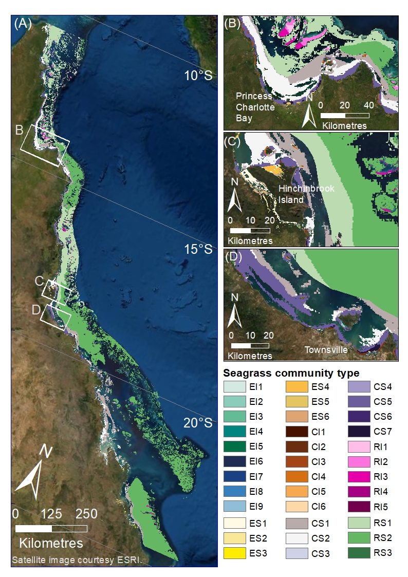
This dataset describes the predicted distribution of seagrass communities across the Great Barrier Reef World Heritage Area and adjacent estuaries, based on six multivariate regressions tree models for estuary intertidal, estuary subtidal, coastal intertidal, coastal subtidal, reef intertidal, and reef subtidal. The models are presented as six raster datasets with 30m resolution. Managing seagrass resources in the GBRWHA requires adequate information on the spatial extent of seagrass communities. The enormous size of the GBRWHA (1000s of kilometres) and the remoteness of many seagrass meadows from human populations means that models are a useful tool to predict where different seagrass communities are likely to be in areas where data is lacking. James Cook University’s Centre for Tropical Water & Aquatic Ecosystem Research (TropWATER) has been collecting spatial data on GBR seagrass since the early 1980s. This project used TropWATER’s synthesis of seagrass site data (NESP Project 3.1 and 5.4: https://eatlas.org.au/data/uuid/5011393e-0db7-46ce-a8ee-f331fcf83a88) to predict seagrass communities. In making this data publically available for management, the authors from the TropWATER Seagrass Group request being contacted and involved in decision making processes that incorporate this data, to ensure its limitations are fully understood. Methods: Seagrass data The sampling methods used to study, describe and monitors seagrass meadows were developed by the TropWATER Seagrass Group and tailored to the location and habitat surveyed; descriptions and references are available in the metadata for the GBRWHA data composite (https://eatlas.org.au/data/uuid/5011393e-0db7-46ce-a8ee-f331fcf83a88). Environmental data Environmental predictors used in the models were: depth below mean sea level (Beaman 2017), relative tidal exposure (Bishop-Taylor et al. 2019), water type (Marine Water Bodies definitions version 2_4, Data courtesy of the Great Barrier Reef Marine Park Authority; Dyall et al. 2004), proportion mud in the sediment (coast and reef models, https://research.csiro.au/ereefs/models/model-outputs/access-to-raw-model-output/) (see also Baird et al. 2020; Margvelashvili et al. 2018), dominant sediment (estuary models only; https://eatlas.org.au/data/uuid/5011393e-0db7-46ce-a8ee-f331fcf83a88), benthic geomorphology (Heap and Harris 2008), benthic light https://dapds00.nci.org.au/thredds/catalog/fx3/gbr1_bgc_924/catalog.html (see also Baird et al. 2016; Baird et al. 2020), water temperature, mean current speed and salinity https://thredds.ereefs.aims.gov.au/thredds/catalog/ereefs/gbr1_2.0/all-one/catalog.html (Steven et al. 2019), wind speed (https://thredds.ereefs.aims.gov.au/thredds/catalog/ereefs/gbr1_2.0/all-one/catalog.html ) and Australian Bureau of Meteorology’s ACCESS data products (Bureau of Meteorology 2020; Soldatenko et al. 2018; Steven et al. 2019), and latitude. Different models had different combinations of predictors after removing collinear variables and excluding variables that did not extend into an area. For example, estuary models only include depth, relative tidal exposure, dominant sediment, and latitude. Models We modelled seagrass communities in six areas: Estuary Intertidal, Estuary Subtidal, Coastal Intertidal, Coastal Subtidal, Reef Intertidal and Reef Subtidal. For each area we used multivariate regression trees to examine changes in seagrass community type within the GBRWHA and adjacent estuaries, using a matrix of seagrass presence/absence site data for 12 seagrass species in the data set. Multivariate regression trees (MRTs) were implemented using the R package mvpart (De’ath 2004) (available in archive form on CRAN at https://cran.r-project.org) in R version 4.0.2 (R Core Team 2020). The map in Figure 1 was created using ArcGIS 10.8. A detailed description of the modelled communities can be found in the final report for the NESP TWQ Project 5.4 (currently in review). Spatial limits Seagrass community types were modelled within potential seagrass habitat. Potential seagrass habitat was modelled by Carter et al. 2020 and is available on eAtlas here: https://eatlas.org.au/data/uuid/108ee868-4fb1-4e5f-ae57-5d65198384cc . The models do not extend north and south of the GBRWHA. The models extend across the continental shelf but exclude waters deeper than ~100m east of the shelf that were not surveyed for seagrass. Data were included when sites extended west of the GBRWHA boundary into coastal and estuarine water immediately adjacent. Data sets The site data used in this model is available here: https://eatlas.org.au/data/uuid/5011393e-0db7-46ce-a8ee-f331fcf83a88) Further information can be found in the upcoming publications of the final report for the NESP TWQ Project 5.4. Limitations of the data: The site data used in these models extends back to the mid-1980s. Large parts of the coast have not been mapped for seagrass presence since that time. The seagrass community rasters are at 30m grid resolution, however some environmental variables such as those from eReefs (wind speed, current speed, benthic light, water temperature) are from spatial data at 1km grid resolution, and are likely to vary at much smaller spatial scales that we could not include in these models. Format: This dataset consists of six raster datasets with a geographic coordinate system of WGS84. The rasters have been saved as layer packages with symbology representing seagrass communities. These are: Estuary intertidal communities: GBR_seagrass_communities_estuary_intertidal.lpk Estuary subtidal communities: GBR_seagrass_communities_estuary_subtidal.lpk Coastal intertidal communities: GBR_seagrass_communities_coastal_intertidal.lpk Coastal subtidal communities: GBR_seagrass_communities_coastal_subtidal.lpk Reef intertidal communities: GBR_seagrass_communities_reef_intertidal.lpk Reef subtidal communities: GBR_seagrass_communities_reef_subtidal.lpk References: TBC Data Location: This dataset is filed in the eAtlas enduring data repository at: data\custodian\2019-2022-NESP-TWQ-5\5.4_Seagrass-Burdekin-region Additional licensing information: TropWATER gives no warranty in relation to the data (including accuracy, reliability, completeness, currency or suitability) and accepts no liability (including without limitation, liability in negligence) for any loss, damage or costs (including consequential damage) relating to any use of the data. TropWATER reserves the right to update, modify or correct the data at any time. The limitations of some older data included need to be understood and recognised. The TropWATER Seagrass Group would appreciate the opportunity to review documents providing research, management, legislative or compliance advice based on this data.

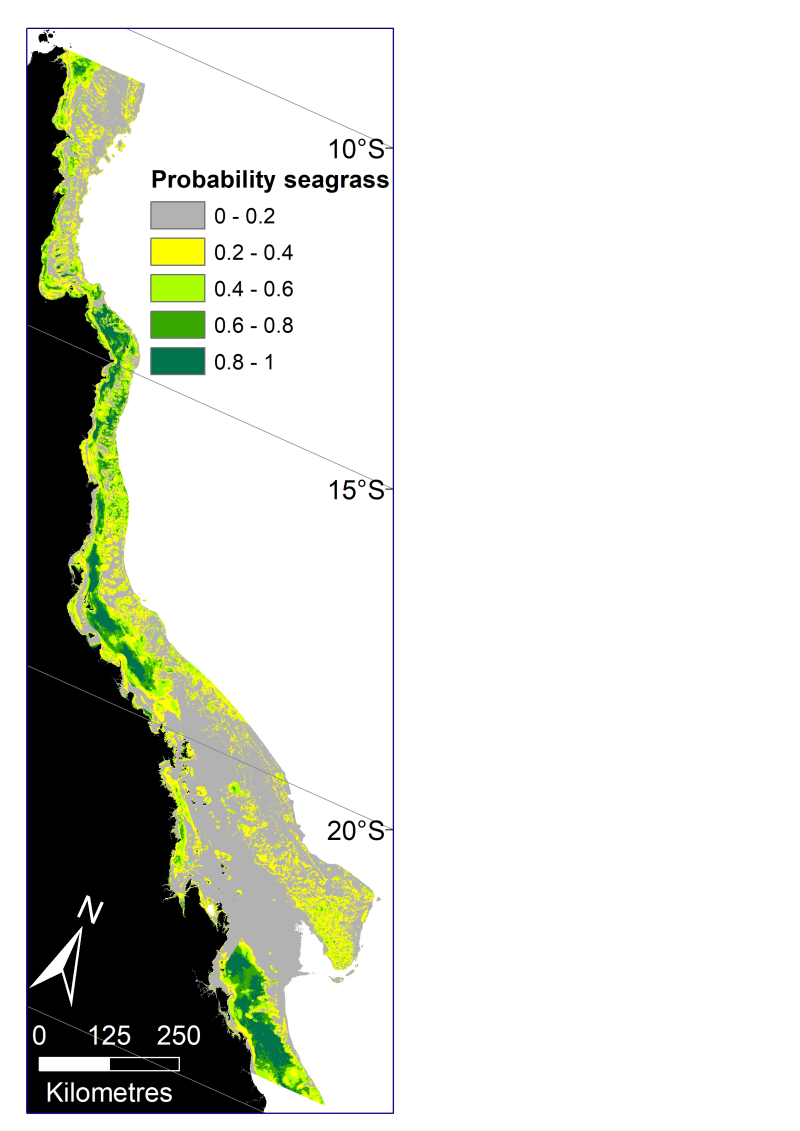
This dataset describes the predicted probability of seagrass presence across the Great Barrier Reef World Heritage Area and adjacent estuaries, based on six Random Forest models. The models have been mosaicked together into one raster dataset with 30m resolution. Managing seagrass resources in the GBRWHA requires adequate information on the spatial extent of seagrass habitat. The enormous size of the GBRWHA (1000s of kilometres) and the remoteness of many seagrass meadows from human populations means that models are a useful tool to predict the probability of seagrass for areas where data is lacking. James Cook University’s Centre for Tropical Water & Aquatic Ecosystem Research (TropWATER) has been collecting spatial data on GBR seagrass since the early 1980s. This project used TropWATER’s synthesis of seagrass site data (NESP Project 3.1 and 5.4: https://eatlas.org.au/data/uuid/5011393e-0db7-46ce-a8ee-f331fcf83a88) to predict potential seagrass habitat. In making this data publically available for management, the authors from the TropWATER Seagrass Group request being contacted and involved in decision making processes that incorporate this data, to ensure its limitations are fully understood. Methods: Seagrass data The sampling methods used to study, describe and monitors seagrass meadows were developed by the TropWATER Seagrass Group and tailored to the location and habitat surveyed; descriptions and references are available in the metadata for the GBRWHA data composite ( https://eatlas.org.au/data/uuid/5011393e-0db7-46ce-a8ee-f331fcf83a88 ). Environmental data Environmental predictors used in the models were: depth below mean sea level (Beaman 2017), relative tidal exposure (Bishop-Taylor et al. 2019), water type (Marine Water Bodies definitions version 2_4, Data courtesy of the Great Barrier Reef Marine Park Authority; Dyall et al. 2004), proportion mud in the sediment (coast and reef models, https://research.csiro.au/ereefs/models/model-outputs/access-to-raw-model-output/ ) (see also Baird et al. 2020; Margvelashvili et al. 2018), dominant sediment (estuary models only; https://eatlas.org.au/data/uuid/5011393e-0db7-46ce-a8ee-f331fcf83a88 ), benthic geomorphology (Heap and Harris 2008), benthic light https://dapds00.nci.org.au/thredds/catalog/fx3/gbr1_bgc_924/catalog.html (see also Baird et al. 2016; Baird et al. 2020), water temperature, mean current speed and salinity https://thredds.ereefs.aims.gov.au/thredds/catalog/ereefs/gbr1_2.0/all-one/catalog.html (Steven et al. 2019), wind speed ( https://thredds.ereefs.aims.gov.au/thredds/catalog/ereefs/gbr1_2.0/all-one/catalog.html ) and Australian Bureau of Meteorology’s ACCESS data products (Bureau of Meteorology 2020; Soldatenko et al. 2018; Steven et al. 2019), and latitude. Different models had different combinations of predictors after removing collinear variables and excluding variables that did not extend into an area. For example, estuary models only include depth, relative tidal exposure, dominant sediment, and latitude. Models We modelled seagrass probability in six areas: Estuary Intertidal, Estuary Subtidal, Coast Intertidal, Coast Subtidal, Reef Intertidal and Reef Subtidal. For each area we used the machine learning technique random forest to broadly examine whether there were habitats within the GBRWHA and adjacent estuaries where seagrass was never likely to grow, using the binary classification within the site data of seagrass present (1) or absent (0) irrespective of species. Random Forest models were implemented using the randomForest package (Liaw and Wiener 2002) in R version 4.0.2 (R Core Team 2020). We used ArcGIS 10.8 to mosaic the six rasters and create a single seagrass probability raster for the GBRWHA. Spatial limits Seagrass data north and south of the GBRWHA were not included in the analysis. The model extends across the continental shelf but excludes waters deeper than ~100m east of the shelf that were not surveyed for seagrass. Data were included when sites extended west of the GBRWHA boundary into coastal and estuarine water immediately adjacent. Data sets The site data used in this model is available here: https://eatlas.org.au/data/uuid/5011393e-0db7-46ce-a8ee-f331fcf83a88 Further information can be found in the upcoming publications of the final report for the NESP TWQ Project 5.4. Limitation of the data: The site data used in these models extends back to the mid-1980s. Large parts of the coast have not been mapped for seagrass presence since that time. The seagrass probability raster is at 30m grid resolution, however some environmental variables such as those from eReefs (wind speed, current speed, benthic light, water temperature) are from spatial data at 1km grid resolution, and are likely to vary at much smaller spatial scales that we could not include in these models. Format: This dataset consists of a raster dataset with a geographic coordinate system of WGS84. The raster has been saved as a layer package with symbology representing seagrass probability in 0.2 increments with a range of 0-1 (GBRWHA_seagrass_probability.lpk) References: TBC Data Location: This dataset is filed in the eAtlas enduring data repository at: data\custodian\2019-2022-NESP-TWQ-5\5.4_Seagrass-Burdekin-region Additional licensing information: TropWATER gives no warranty in relation to the data (including accuracy, reliability, completeness, currency or suitability) and accepts no liability (including without limitation, liability in negligence) for any loss, damage or costs (including consequential damage) relating to any use of the data. TropWATER reserves the right to update, modify or correct the data at any time. The limitations of some older data included need to be understood and recognised. The TropWATER Seagrass Group would appreciate the opportunity to review documents providing research, management, legislative or compliance advice based on this data.

This dataset consists of monitoring data from macroalgae removal and larval seeding experiments in Florence and Arthur Bay at Magnetic Island, Queensland, Australia, collected between 2018-2020. There were twelve 5x5m permanent plots in each bay; three with macroalgae removal only, three with larval seeding only, three with macroalgae removal and larval seeding and three control plots. These data include: - Stationary point count fish survey data - Photo quadrats - Coral recruitment to settlement tiles - Macroalgae frond height, holdfast presence and biomass removed **This dataset is currently under embargo. The first phase of the project (2018-2019) was macroalgae removal only, with six permanent plots in each bay (three removal, and three controls). The second phase, beginning in July 2019, included six additional plots in each bay (n=12 plots per bay) and an additional experimental treatment in Arthur Bay only, where settlement-ready coral larvae were added to six of the plots per bay (n=3 plots per treatment). In Florence Bay, upon addition of the six new plots, the six original plots were re-assigned within the algal removal treatments (n=6 plots per treatment). Original plots in Arthur Bay maintained their designation of removal / non-removal, and these designations were then superimposed with larvae / no larvae. Methods: - Fish surveys: Fifteen-minute stationary point counts (SPC) with all fish present recorded, followed by a cryptic crawl (CC) consisting of five-minute search for additional species within the plot. Data was collected from March 2019 to February 2020 (4 surveys). - Photos: Three quadrats in each bay were randomly assigned for macroalgae removal and the remaining three were left untouched, representing control quadrats. Each quadrat was divided into 25 squares (1x1 m) using transect tapes, which form a gridline formation, and these squares were photographed using a digital camera at a distance of approximately 1 m above the region of interest at each survey time point. Reef benthic monitoring photographs were obtained at all quadrats (n=12) prior to macroalgae removal as a baseline in October 2018 and were recorded again immediately after manual removal of macroalgae from three of the quadrats in each bay (n=6). Four subsequent reef monitoring photograph surveys were conducted between November 2018 and May 2019. A total of 1650 photographs were obtained for this survey period. - Natural Recruits: Within the twenty-four 5x5m plots, three replicate 1x1m quadrats were haphazardly placed. All coral recruits up to 4cm were counted within the 1m2 quadrat and categorised as “branching” or “other” morphology. Recruits were also measured and categorised by diameter (i.e. 0-1cm, 1-2cm, 2-3cm, and 3-4cm). For treatment (i.e. algal removal) plots, this process was completed both before and after algal removal. - Recruit and lab reared tiles: Terra cotta tiles were used as a proxy for bare substrate, and were installed on the reef approximately 6 weeks prior to the mass spawning event in 2018 and 2019. Following the 2018 spawning, tiles were removed at two time points – February and March 2019 – to assess recruitment success and growth between control and removal plots. Upon removal, tiles were soaked for 48 hours in a 5% sodium hypochlorite solution. Coral skeletons were counted, measured, and photographed using a Nikon SMZ745T photo-microscope. Prior to the 2019 spawning, twenty adult coral colonies were removed from Horseshoe Bay, Magnetic Island and used as broodstock. These twenty colonies were maintained in aquaria at the National Sea Simulator at AIMS. Their spawn was collected, allowed to fertilise, and cultured in aquaria for 5 days. The competent larvae were released into specialised underwater tents into each of six treatment plots (3 with algal removal, 3 without) in Arthur Bay. An initial settlement check was performed by removing the settlement tiles and examining them under a microscope, counting all recruits, and placing the tiles back into the plots. Recruit counts were repeated in February and October 2020. - Macroalgae: Three 1x1m squares were haphazardly selected within each plot and the total number of macroalgae holdfasts recorded by divers. Algal height was measured for 10 algal fronds (from holdfast to end of frond). Biomass was the wet weight of algae removed from the removal plots. Limitations of the data: - Fish: Surveys were only done during daylight hours, so nocturnal fish are likely to have been missed, visibility was low at times making it harder to see fish, cryptic fishes are often missed during visual surveys. - Photo quadrats: Algae canopy can make it difficult to estimate benthic cover, ID challenges in general, low visibility makes it challenging to get clear photos. - Recruits: Bleaching method doesn’t allow to see if a recruit was alive when sampled; settlement tiles are not exact analogues to natural reef environment; some tiles were lost or tampered with. - Algae: Macroalgae were not identified to species level, it can be hard to define what a holdfast is. Format: This dataset consists of four spreadsheets datasets associated with the ecology and community composition of the experiments. 1_Fish_Data Fish community data from underwater surveys 2_Photo_Quadrats Photos showing benthic cover (coral, macroalgae etc.) within experimental plots 4_Natural_Recruits Coral recruits to tiles within experimental plots without larval seeding 5_Recruit&Lab-reared_Tiles Coral recruits to tiles for the larvae seeding experiments 6_Macroalgae Macroalgae frond height, number of holdfasts and biomass of removed macroalgae Data Dictionary: Fish surveys: File: Fish - macroalgae removal experiments magnetic island.xlsx [2 datasheets: Stationary Point Count (SPC) & Cryptic Crawl (CC)] - Date: Date of survey - Time: Survey start time - Bay: Two sites on Magnetic Island were surveyed - Arthur and Florence Bays - Plot: Fixed plot number surveyed at each of 2 sites - Treatment: Control, Removal only, Larvae, Removal and larvae - ID: sample/quadrat photo ID - Visibility (m): water visibility assessed by diver at start of dive - Species: Fish species observed - Count: Total number of fish of each species observed - Observer: Name of diver recording fish data Natural Recruits: *Note that this part of monitoring commenced in the “Study” phase, so no pilot data exists (nor does the column specifying study phase) File name: Recruits.csv - LOCATION: Two sites on Magnetic Island - Arthur and Florence Bays - PLOT: Fixed plot number surveyed at each of 2 sites - DATE: Date of survey - QUADRAT: Replicate 1x1m square quadrat within each experimental plot - TREATMENT: Treatment, macroalgae removal, larval enhancement, both or none. - PRE-POST: when the survey was conducted, either pre- or post-removal of algae - SIZE: categories of recruit diameter where 1=0-1cm; 2 = 1-2cm; 3 = 2-3cm, 4 = 3-4cm - MORPHOLOGY - COUNT: number of coral recruits observed - OBSERVER: The person who made the observation Lab-reared recruits: File name: LabRearedRecruits.xlsx [2 datasheets: Treatment & Control] - Sort: Individual identifier - Plot: Plot number - Treatment: Experimental treatment - Tile: Tile number - Surface: side of the tile where recruits were counted - Acroporidae: Number of recruits from the family Acroporidae - Total per tile: Total number of coral recruits per tile - Mean per tile plot: Mean number of coral recruits per tile within a plot - Mean per tile: Mean number of coral recruits per tile - Pocilloporidae: Number of recruits from the family Pocilloporida - Others: Number of coral recruits from other families Macroalgae: File name: Holdfasts.csv - BAY Two sites on Magnetic Island - Arthur and Florence Bays - PLOT Fixed plot number surveyed at each of 2 sites - HOLDFASTS The number of Sargassum holdfasts counted in each 1x1m replicate - DATE: date of survey - TREATMENT: Treatment of macroalgae removal, larval enhancement, both or none. - PRE/POST: when the survey was conducted, either pre- or post-removal of algae - OBSERVER: the person making the observation - STUDY-PHASE: either Pilot or Study. Pilot phase included 6 plots per bay, while Study phase included 12 plots per bay. Furthermore the plot treatment designations were changed in Florence Bay between Pilot and Study phases. - NOTES: miscellaneous text File name: Biomass.xlsx - BAY: Two sites on Magnetic Island – Arthur and Florence Bays - PLOT: Fixed plot number surveyed at each of 2 sites - DATE: date of survey - TREATMENT: Treatment of macroalgae removal, larval enhancement, both, or none - KG: Kilograms of wet weight macroalgae removed from each experimental plot, weighed to the nearest 0.1kg using fish scales. - OBSERVER: The person making the observation File name: Algae.csv - BAY: Two sites on Magnetic Island – Arthur and Florence Bays - PLOT: Fixed plot number surveyed at each of 2 sites - QUADRAT: Replicate 1x1m quadrat within each plot being surveyed. Three replicates per plot. - FROND: Replicate number of frond measurement, 1-10 - HEIGHT: Height of the algal frond from holdfast to frond tip, measured in cm. - DATE: Date of survey - TREATMENT: Treatment of macroalgae removal, larval enhancement, both, or none - PrePostRemoval: when the survey was conducted, either pre- or post-removal of algae - OBSERVER: the person making the observation - STUDY-PHASE: either Pilot or Study. Pilot phase included 6 plots per bay, while Study phase included 12 plots per bay. Furthermore the plot treatment designations were changed in Florence Bay between Pilot and Study phases. - NOTES: any miscellaneous text Data Location: This dataset is filed in the eAtlas enduring data repository at: data\nesp4\4.3_Best-practice-coral-restoration\

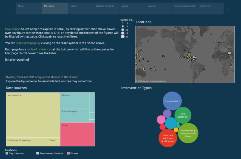
This dataset consists of a review of case studies and descriptions of coral restoration methods from four sources: 1) the primary literature (i.e. published peer-reviewed scientific literature), 2) grey literature (e.g. scientific reports and technical summaries from experts in the field), 3) online descriptions (e.g. blogs and online videos describing projects), and 4) an online survey targeting restoration practitioners (doi:10.5061/dryad.p6r3816). Included are only those case studies which actively conducted coral restoration (i.e. at least one stage of scleractinian coral life-history was involved). This excludes indirect coral restoration projects, such as disturbance mitigation (e.g. predator removal, disease control etc.) and passive restoration interventions (e.g. enforcement of control against dynamite fishing or water quality improvement). It also excludes many artificial reefs, in particular if the aim was fisheries enhancement (i.e. fish aggregation devices), and if corals were not included in the method. To the best of our abilities, duplication of case studies was avoided across the four separate sources, so that each case in the review and database represents a separate project. Methods: More than 40 separate categories of data were recorded from each case study and entered into a database. These included data on (1) the information source, (2) the case study particulars (e.g. location, duration, spatial scale, objectives, etc.), (3) specific details about the methods, (4) coral details (e.g. genus, species, morphology), (5) monitoring details, and (6) the outcomes and conclusions. Primary literature Multiple search engines were used to achieve the most complete coverage of the scientific literature. First, the scientific literature was searched using Google Scholar with the keywords “coral* + restoration”. Because the field (and therefore search results) are dominated by transplantation studies, separate searches were then conducted for other common techniques using “coral* + restoration + [technique name]”. This search was further complemented by using the same keywords in ISI Web of Knowledge (search yield n=738). Studies were then manually selected that fulfilled our criteria for active coral restoration described above (final yield n= 221). In those cases where a single paper describes several different projects or methods, these were split into separate case studies. Finally, prior reviews of coral restoration were consulted to obtain case studies from their reference lists. Grey literature While many reports appeared in the Google Scholar literature searches, The Nature Conservancy (TNC) database of reports for North American coastal restoration projects (http://projects.tnc.org/coastal/) was also conducted. This was supplemented with reports listed in the reference lists of other papers, reports and reviews, and during the online searches (n=30). Online records Small-scale projects conducted without substantial input from researchers, academics, non-governmental organisations (NGO) or coral reef managers often do not result in formal written accounts of methods. To access this information, we conducted online searches of YouTube, Facebook and Google, using the search terms “Coral restoration”. The information provided in videos, blog posts and websites to describe further projects (n=48) was also used. Due to the unverified nature of such accounts, the data collected from these online-only records was limited compared to peer reviewed literature and surveys. At the minimum, the location, the methods used and reported outcomes or lessons learned were included in this review. Online survey To access information from projects not published elsewhere, an online survey targeting restoration practitioners was designed. The survey consisted of 25 questions querying restoration practitioners regarding projects they had undertaken under JCU human ethics H7218 (following the Australian National Statement on Ethical Conduct in Human Research, 2007). These data (n=63) are included in all calculations within this review, but are not publicly available to preserve the anonymity of participants. Although we encouraged participants to fill out a separate survey for each case study, it is possible that participants included multiple separate projects in a single survey, which may reduce the real number of case studies reported. Data analysis Percentages, counts and other quantifications from the database refer to the total number of case studies with data in that category. Case studies where data were lacking for the category in question, or lack appropriate detail (e.g. reporting ‘mixed’ for coral genera) are not included in calculations. Many categories allowed multiple answers (e.g. coral species); these were split into separate records for calculations (e.g. coral species n). For this reason, absolute numbers may exceed the number of case studies in the database. However, percentages reflect the proportion of case studies in each category. We used the seven objectives outlined in [1] to classify the objective of each case study, with an additional two categories (‘scientific research’ and ‘ecological engineering’). We used Tableau to visualise and analyse the database (Desktop Professional Edition, version 10.5, Tableau Software). The data have been made available following the FAIR Guiding Principles for scientific data management and stewardship [2]. Data available from the Dryad Digital Repository downloaded here (https://doi.org/10.5061/dryad.p6r3816), and visually explored: https://public.tableau.com/views/CoralRestorationDatabase-Visualisation/Coralrestorationmethods?:embed=y&:display_count=yes&publish=yes&:showVizHome=no#1. Limitations: While our expanded search enabled us to avoid the bias from the more limited published literature, we acknowledge that using sources that have not undergone rigorous peer-review potentially introduces another bias. Many government reports undergo an informal peer-review; however, survey results and online descriptions may present a subjective account of restoration outcomes. To reduce subjective assessment of case studies, we opted not to interpret results or survey answers, instead only recording what was explicitly stated in each document [3, 4]. Defining restoration In this review, active restoration methods are methods which reintroduce coral (e.g. coral fragment transplantation, or larval enhancement) or augment coral assemblages (e.g. substrate stabilisation, or algal removal), for the purposes of restoring the reef ecosystem. In the published literature and elsewhere, there are many terms that describe the same intervention. For clarity, we provide the terms we have used in the review, their definitions and alternative terms (see references). Passive restoration methods such as predator removal (e.g. crown-of-thorns starfish and Drupella control) have been excluded, unless they were conducted in conjunction with active restoration (e.g. macroalgal removal combined with transplantation). Format: The data is supplied as an excel file with three separate tabs for 1) peer reviewed literature 2) grey literature, and 3) a description of the objectives form Hein et al. 2017. Survey responses have been excluded to preserve the anonymity of the respondents. This dataset is a database that underpins a 2018 report and 2019 published review of coral restoration methods from around the world. - Bostrom-Einarsson L, Ceccarelli D, Babcock R.C., Bayraktarov E, Cook N, Harrison P, Hein M, Shaver E, Smith A, Stewart-Sinclair P.J, Vardi T, McLeod I.M. 2018 - Coral restoration in a changing world - A global synthesis of methods and techniques, report to the National Environmental Science Program. Reef and Rainforest Research Centre Ltd, Cairns (63pp.). - Review manuscript is currently under review. Data Dictionary: The Data Dictionary is emended in the excel spreadsheet. Comments are included in the column titles to aid interpretation, and/or refer to additional information tabs. For more information on each column, open the red triangle [located top right of cell]. References: 1. Hein MY, Willis BL, Beeden R, Birtles A. The need for broader ecological and socioeconomic tools to evaluate the effectiveness of coral restoration programs. Restoration Ecology. Wiley/Blackwell (10.1111); 2017;25: 873–883. doi:10.1111/rec.12580 2. Wilkinson MD, Dumontier M, Aalbersberg IJ, Appleton G, Axton M, Baak A, et al. The FAIR Guiding Principles for scientific data management and stewardship. Scientific Data 2016 3. Nature Publishing Group; 2016;3: 160018. doi:10.1038/sdata.2016.18 3.Miller RL, Marsh H, Cottrell A, Hamann M. Protecting Migratory Species in the Australian Marine Environment: A Cross-Jurisdictional Analysis of Policy and Management Plans. Front Mar Sci. Frontiers; 2018;5: 211. doi:10.3389/fmars.2018.00229 4. Ortega-Argueta A, Baxter G, Hockings M. Compliance of Australian threatened species recovery plans with legislative requirements. Journal of Environmental Management. Elsevier; 2011;92: 2054–2060. Data Location: This dataset is filed in the eAtlas enduring data repository at: data\2018-2021-NESP-TWQ-4\4.3_Best-practice-coral-restoration